- Download
- Welcome to SOFiA
- Who is behind SOFiA
- Feature overview
- System overview
- Function reference
- readVSAdata
- mergeArrayData
- F/D/T
- gauss
- lebedev
- S/W/G
- S/T/C
- W/G/C
- S/F/E
- M/F
- R/F/I
- P/D/C
- I/T/C
- makeMTX
- makeIR
- visual3D
- Coordinate System
- Application Examples
- Example 1
- Example 2
- Example 3
- Example 4
- Example 5
- Example 6
- Example 7
- Example 8
- Array Datasets
- VariSphear system
- Groups and Mailinglists
- Contact and Support
- How to Reference
|
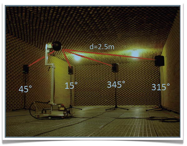
SOFiA application example 5
This example shows 4 "plane waves" impinging to a real array in a rigid sphere configuration that arrive at different times. We work on a real array dataset: EXAMPLE 3. The four sources have the same level but different time delays (45°:0ms, 15°:16ms, 345°:32ms, 315°:48ms). This example shows how to get access to the spatiotemporal sound field information running a plane wave decomposition on different time windows.
File(s)
Run `sofiaAE5.m`.
Locate the folder `EXAMPLE3_SpatioTemporal` containing the required array data.
Output

Take care: This figure shows frontal views of the array response and the photo on top shows the rear side of the array.
Code
/*
% SOFiA example 5: Spatiotemporal resolution
% SOFiA Version : R11-1220
% Array Dataset : R11-1018
clear all
clc
% Read VariSphear dataset
% !!! LOCATE THE FOLDER: "EXAMPLE2_LevelResolution"
timeData = sofia_readVSAdata();
|
|
|
figure(2) % Enable to get an IR overview
clf();
area(timeData.irOverlay');
fftOversize = 2;
startSample = [400 1100 1800 2500]; % Examplary values (Enable area plot)
blockSize = 256;
figure(1)
clf();
for ctr=1:size(startSample, 2)
% Here we have simply put a loop around, because this is good for
% understanding this experiment. The loop content can easily be optimized.
% Transform time domain data to frequency domain and generate kr-vector
[fftData, kr, f] = sofia_fdt(timeData, fftOversize, startSample(ctr), startSample(ctr)+blockSize);
% Spatial Fourier Transform
Nsft = 5;
Pnm = sofia_stc(Nsft, fftData, timeData.quadratureGrid);
|
% Radial Filters for a rigid sphere array
Nsft = 5;
Pnm = sofia_stc(Nsft, fftData, timeData.quadratureGrid);
% Radial filters for a rigid sphere array
Nrf = Nsft; % radial filter order
maxAmp = 10; % Maximum modal amplification in [dB]
ac = 2; % Array configuration: 2 0 Rigid Sphere
dn = sofia_mf(Nrf, kr, ac, maxAmp); % radial filters
% Make MTX
Nmtx = Nsft;
krIndex = 90; % Choose the kr-bin (Frequency) to display.
mtxData = sofia_makeMTX(Nmtx, Pnm, dn, krIndex);
subplot(2, 2, ctr);
sofia_visual3D(mtxData, 0);
view(90, 0)
end
disp(The plot shows the response at a frequency of ',num2str(round(10*f(krIndex))/10),'Hz');
|
*/ |
|
|

