- Download
- Welcome to SOFiA
- Who is behind SOFiA
- Feature overview
- System overview
- Function reference
- readVSAdata
- mergeArrayData
- F/D/T
- gauss
- lebedev
- S/W/G
- S/T/C
- W/G/C
- S/F/E
- M/F
- R/F/I
- P/D/C
- I/T/C
- makeMTX
- makeIR
- visual3D
- Coordinate System
- Application Examples
- Example 1
- Example 2
- Example 3
- Example 4
- Example 5
- Example 6
- Example 7
- Example 8
- Array Datasets
- VariSphear system
- Groups and Mailinglists
- Contact and Support
- How to Reference
|
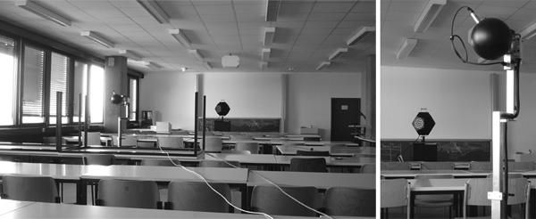
SOFiA application example 8
In this example we render directional impulse responses from real array measurement data taken in a classroom, Array Example 5. The original array data recorded at 44.1KHz is downsampled to 22.05KHz to avoid spatial aliasing. Later the IRs are resampled to 44.1KHz again (but of course there is no information >11KHz anymore!). The transform and decomposition orders are N=4 and we allow a maximum modal amplification of 10dB in this example.
File(s)
Run `sofiaAE8.m`.
Locate the folder `EXAMPLE5_RealRoom` containing the required array data.
Output

Code
/*
% SOFiA example 8: Superdirective impulse responses
% SOFiA Version : R11-1220
% Array Dataset : R11-1018
clear all
clc
% Read VariSphear dataset
% !!! LOCATE THE FOLDER: "EXAMPLE5_RealRoom"
downsample = 2;
timeData = sofia_readVSAdata(downsample);
|
[fftData, kr, f] = sofia_fdt(timeData);
% Spatial Fourier Transform
Nsft = 4;
Pnm = sofia_stc(Nsft, fftData, timeData.quadratureGrid);
% Radial Filters for a rigid sphere array
Nrf = Nsft; % radial filter order
maxAmp = 10; % Maximum modal amplification in [dB]
ac = 2; % Array configuration: 2 = Rigid Sphere
dn = sofia_mf(Nrf , kr, ac, maxAmp);
[dn, kernelSize, latency] = sofia_rfi(dn);
% Plane wave decomposition for directions given by OmegaL:
Npdc = Nsft; Plane wave decomposition order
OmegaL = 0 pi/2; pi pi/2;
Y = sofia_pdc(Npdc, OmegaL, Pnm, dn);
% Reconstruct directional impulse responses
impulseResponses = sofia_makeIR(Y, 1/8, downsample);
% Remove filter latency (Be careful; this is done very roughly here
% for demonstration/visualisation purpose only)
impulseResponses = impulseResponses(:, (latency*downsample):end);
figure(1)
tscale = linspace(0,size(impulseResponses,2)/(timeData.FS*downsample), size(impulseResponses,2));
plot(tscale, impulseResponses')
title('Directional Impulse Responses')
xlabel('Time in s')
ylabel('Signal Amplitude'
|
Make MTX
Nmtx = Nsft;
krIndex = 90;
mtxData = sofia_makeMTX(Nmtx; Pnm; dn; krIndex);
Nrf = Nsft;
maxAmp = 10;
ac = 2;
dn = sofia_mf(Nrf ; kr; ac; maxAmp)
;
subplot(2; 2; ctr);
sofia_visual3D(mtxData; 0);
view(90; 0)
end
disp(The plot shows the response at a frequency of ',num2str(round(10*f(krIndex))/10),'Hz');
|
Maximum modal amplification in [dB]
Array configuration: 2 = Rigid Sphere
radial filters
*/ |
|
|

